Realizing Efficiency in Data Analysis in Microsoft Excel 2013: A Pivot Table Primer

I often debate with other Microsoft Excel Wizards about the merit of Pivot Tables over formulas.  I’m struck by how vehemently some people oppose their use, preferring Nested If fun that can take hours to get right over a few clicks to arrive at the same answer.

I’m not a Pivot Table purist by any means.  I enjoy the mental challenge that comes with deciphering Microsoft Excel’s sometimes maddening parenthesis patterns and “coding” my spreadsheet every now and then.  And I am proud of the fact that I don’t have to go running to the office next to mine for help with a particularly nasty Nested If statement anymore. 

But if you don’t know about and use Pivot Tables, you really really should.  They save time, and, unlike formulas, are malleable to allow you to slice and dice your data.  Let’s look at a quick example of formulas vs.  a Pivot Table.

One quick disclaimer.  Microsoft Excel is a very robust tool.    You can even go behind the curtains and write your own VB if you really want to.  There are keyboard shortcuts, many many different ways to Insert cells, write formulas, and parse data.  What I am about to show is not the only way to create this analysis; indeed, it may not even be the best way to do it.  I don't however think that it can be argued that what I am about to demonstrate are common methods of working within Excel. I ask the Excel Wizards to accept that for the sake of this discussion.  Lastly, I use Microsoft Excel 2013, and all of my commands, menus, etc. reflect the use of that version.

Here's a simple spreadsheet tracking the hours of four people over a period of time.  In Excel, terms, this is about as simple as a multi-column spreadsheet gets, yet it contains some very pertinent information if you use it as the starting point for some data analysis:

OK, so let's say I want to roll-up my hours for each person and get a grand total for the entire group.  I can use formulas to do this, such as:  SUMIF(A:A,"bob",C:C); writing the formula or copy/pasting it three more times and substituting "bob:" with the names of the other guys in the list.    To get my sum total for the group, I can use another formula, like:  =SUM(F2:F5).  Toss in some minor formatting as well as data headers and the end product looks like this:

Not too bad, right?  Start to finish, this probably took me  something like two minutes to create. I have my data and I have my analysis.  Let's go have a beer to celebrate!

One moment please.  Let's try a Pivot Table.  To start, we go Insert->Pivot Table.  A new window pops up asking a couple of questions.  First, we specify our range and then  tell Excel where to put the Pivot Table:

When I click OK, I get this:

I have a place for my table and I have Options to the right of what to include in it.  To get my total by person and sum overall, first, on the right side, I click Name and I drag it to Row, then I click Hours Billed and I drag it to values:

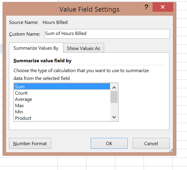
Not quite right, though it is.  That's simply because the Pivot Table by default uses the COUNT function.,  To change it to Sum, we just have to right click on the header and click Sum:

A couple of clicks later and here's the result.  At this point I'll also want to set my sort choice, I do

this by clicking on Row Labels and choosing my sort option.  Note that I could also sort on Hours Billed if I wanted to:

Start to finish, the Pivot Table takes about a minute to create, or half the time that the formulas did.  Bear in mind that this is a simple example,  Imagine dozens of people and hundreds of lines to calculate.  The beauty of the Pivot Table is that were it to take you to create formulas for those dozens of people and it took 15 minutes, your Pivot Table will take...

About a minute still.

Let's look at a couple of other simple features of Pivot Tables.  Say that my team of four becomes a team of five.  I want to add Daryl to my analysis, and I want it to look nice- keep the guys in alphabetical order and such.  

 With my formula I need to:

1. Insert a row between Chris and Frank
2. Type Daryl
3. Insert my SumIf formula 

With my Pivot Table, I need to:

1. Go to Data->Refresh All

The Pivot Table will add Daryl in to its analysis, alphabetically:

. 

Neat, huh?

One more example for the day.  Let's say that I want my analysis to go week over week- list out the hours by person for each week, with a sum total at the end.

Given the way that the data is laid out right now, there's no easy way to change it with my formula example.  Off the top of my head, I could:

1. Create headers across the top with each week.
2. Either manually retype the values in for each person or each week OR do a referential formula to grab the values for you in a little less time.
3. Create a Sum field for each week.

I get it, with this example, its not too much work.  5 minutes on the outside.  Let's compare that level of effort to what a Pivot Table requires.

To get the same result with a Pivot Table I:

1. Click on the Pivot Table to bring up the Fields Menu on the right of the screen.
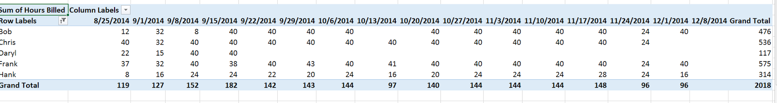
2. Click on Week Of and drag it to the Columns Area

5 seconds on the outside.  Here's what the end result looks like:

Come on, even the most Wizardly of Excel Wizards has to admit that's damn cool.

Hopefully you've seen the value of Pivot Tables within Microsoft Excel.  Give one a try next time you're wanting to do some analysis.  With a little bit of practice you will have an awesome new tool in your arsenal- and bear in mind that I have barely scratched the surface of what Pivot Tables can do.  

Epilogue

I do feel like I need to show some street cred here when it comes to formulas lest I be called a Pivot Table Poser.  Here's some Nested If hell that I whipped up to stretch my muscles a few months ago.  Truth be told though as you'll see even here I used a Pivot Table.  Think about that for a second and imagine what could happen if you took the chocolate of your formulas and combined it with the peanut butter of my Pivot Tables...

=IF(O1="week 1",1/14*N3*GETPIVOTDATA("Hours Billed",$F$2,"Name","Bob")/40,IF(O1="week 2",2/14*$O$3*GETPIVOTDATA("Hours Billed",$F$2,"Name","Bob")/80,IF(O1="week 3",3/14*N3*GETPIVOTDATA("Hours Billed",$F$2,"Name","Bob")/120,IF(O1="week 4",4/14*N3*GETPIVOTDATA("Hours Billed",$F$2,"Name","Bob")/160,IF(O1="week 5",5/14*N3*GETPIVOTDATA("Hours Billed",$F$2,"Name","Bob")/200,IF(O1="week 6",6/14*N3*GETPIVOTDATA("Hours Billed",$F$2,"Name","Bob")/240,IF(O1="week 7",7/14*N3*GETPIVOTDATA("Hours Billed",$F$2,"Name","Bob")/280,IF(O1="week 8",8/14*N3*GETPIVOTDATA("Hours Billed",$F$2,"Name","Bob")/320,IF(O1="week 9",9/14*N3*GETPIVOTDATA("Hours Billed",$F$2,"Name","Bob")/360,IF(O1="week 10",10/14*N3*GETPIVOTDATA("Hours Billed",$F$2,"Name","Bob")/400,IF(O1="week 11",11/14*N3*GETPIVOTDATA("Hours Billed",$F$2,"Name","Bob")/440,IF(O1="week 12",12/14*N3*GETPIVOTDATA("Hours Billed",$F$2,"Name","Bob")/480,IF(O1="week 13",13/14*N3*GETPIVOTDATA("Hours Billed",$F$2,"Name","Bob")/520,IF(O1="week 14",14/14*N3*GETPIVOTDATA("Hours Billed",$F$2,"Name","Bob")/560))))))))))))))